Xlookup is the long awaited improvement on Vlookup, Hlookup and Index Match. It also allows for easier formula writing to allow for matches, Errors and Summing multiple array lookups.
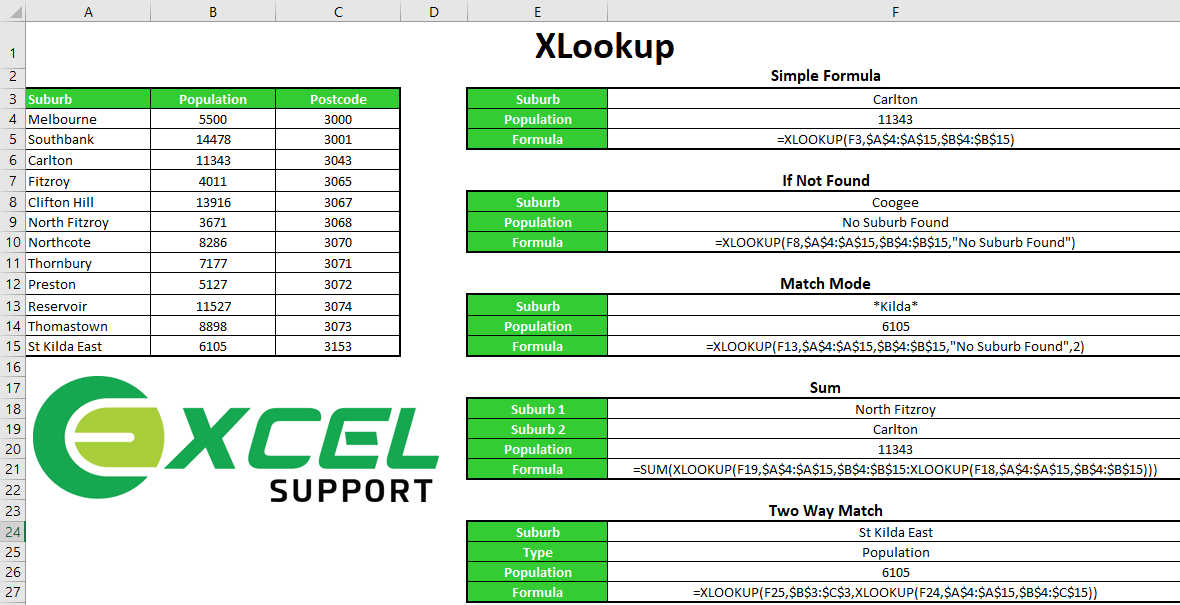
Below are 5 ways to utilise the Xlookup function and the formulas associated.

Xlookup is the long awaited improvement on Vlookup, Hlookup and Index Match. It also allows for easier formula writing to allow for matches, Errors and Summing multiple array lookups.
Below are 5 ways to utilise the Xlookup function and the formulas associated with them.
- Simple Formula using Xlookup
The most straight forward function where we take the lookup value, then the range in which we want to find it in and then finally the result we want to display.
Formula
=XLOOKUP(F3,$A$4:$A$15,$B$4:$B$15)
- If not Found using Xlookup
Previously we would use Iferror to stipulate if something is not found, with Xlookup you can now simply place this within the formula. Be careful if you supply an empty string (“”) for not_found. If no match is found, XLOOKUP will display nothing instead of #N/A. If you want to see the #N/A error when a match isn’t found, omit the argument entirely.
Formula
=XLOOKUP(F8,$A$4:$A$15,$B$4:$B$15,”No Suburb Found”)
- Match Mode using Xlookup
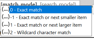
Similar to previous match functions where we were able to stipulate if we wanted an Exact match or not Xlookup allows 4 match types (below).

The example here allows for a wildcard match where the value in F13 has a * before and after it
Formula
=XLOOKUP(F13,$A$4:$A$15,$B$4:$B$15,”No Suburb Found”,2)
- Sum Arrays using Xlookup
Summing the result of two array functions used to be quite cumbersome using Sumproduct or multiple sumifs. With Xlookup it is now way easier. The simple lookup used twice with a “:” between it and wrap a sum function around it.
Formula
=SUM(XLOOKUP(F19,$A$4:$A$15,$B$4:$B$15:XLOOKUP(F18,$A$4:$A$15,$B$4:$B$15)))
- Two Way Match using Xlookup
In our opinion this is the best feature of Xlookup as it eliminates the need to mix lookup and match functions or a number of other workarounds for a simple two way lookup.
In the first section the lookup value will be what Column Header you want to return from. Then stipulate the range, the second section is the same as the Simple formula in Point 1.
Formula
=XLOOKUP(F25,$B$3:$C$3,XLOOKUP(F24,$A$4:$A$15,$B$4:$C$15)
